Deboning linear regression output in Excel

A while back (https://goo.gl/1W11Zu), I outlined interpretation of the output of a multiple linear regression of data on Seattle area housing prices (https://www.kaggle.com/harlfoxem/housesalesprediction?login=true), which provides a convenient way to illustrate the usual output of a multiple linear regression model output in R. This is a 21K dataset with 19 variables on housing characteristics and sales price. It’s a cruddy model, used solely to pick apart the different data presented. Today, it’s Excel’s turn.

Disclosure: I’m not a fan of GUI for most applications. I find it slower and more error prone. Doing this replication elicited the usual grumbles, along with annoyance that multiple independent variables had to be in adjoining columns. Not hard to do, but … .

For comparison, here is the output from the R example, with the addition of an analysis of variance (ANOVA) table that Excel provides by default, but R doesn’t.

library(readr)
library(knitr)
library(kableExtra)
print("Data Structure")

## [1] "Data Structure"

house <- read_csv('https://tuva.s3-us-west-2.amazonaws.com/kc_house_data.csv',comment = '')

## Parsed with column specification:
## cols(
##   .default = col_double(),
##   id = col_character(),
##   date = col_datetime(format = "")
## )

## See spec(...) for full column specifications.

spec(house)

## cols(
##   id = col_character(),
##   date = col_datetime(format = ""),
##   price = col_double(),
##   bedrooms = col_double(),
##   bathrooms = col_double(),
##   sqft_living = col_double(),
##   sqft_lot = col_double(),
##   floors = col_double(),
##   waterfront = col_double(),
##   view = col_double(),
##   condition = col_double(),
##   grade = col_double(),
##   sqft_above = col_double(),
##   sqft_basement = col_double(),
##   yr_built = col_double(),
##   yr_renovated = col_double(),
##   zipcode = col_double(),
##   lat = col_double(),
##   long = col_double(),
##   sqft_living15 = col_double(),
##   sqft_lot15 = col_double()
## )

mod <- lm(price ~ bedrooms + bathrooms + sqft_living + sqft_lot + yr_built, data = house)
summary(mod)

## 
## Call:
## lm(formula = price ~ bedrooms + bathrooms + sqft_living + sqft_lot + 
##     yr_built, data = house)
## 
## Residuals:
##      Min       1Q   Median       3Q      Max 
## -1784413  -131451   -16905   100357  3933748 
## 
## Coefficients:
##               Estimate Std. Error t value Pr(>|t|)    
## (Intercept)  6.006e+06  1.298e+05  46.281   <2e-16 ***
## bedrooms    -7.096e+04  2.246e+03 -31.592   <2e-16 ***
## bathrooms    8.114e+04  3.730e+03  21.755   <2e-16 ***
## sqft_living  3.044e+02  2.998e+00 101.544   <2e-16 ***
## sqft_lot    -3.388e-01  4.119e-02  -8.225   <2e-16 ***
## yr_built    -3.057e+03  6.686e+01 -45.730   <2e-16 ***
## ---
## Signif. codes:  0 '***' 0.001 '**' 0.01 '*' 0.05 '.' 0.1 ' ' 1
## 
## Residual standard error: 245800 on 21607 degrees of freedom
## Multiple R-squared:  0.552,  Adjusted R-squared:  0.5519 
## F-statistic:  5325 on 5 and 21607 DF,  p-value: < 2.2e-16

anova(mod)

## Analysis of Variance Table
## 
## Response: price
##                Df     Sum Sq    Mean Sq   F value    Pr(>F)    
## bedrooms        1 2.7696e+14 2.7696e+14  4585.896 < 2.2e-16 ***
## bathrooms       1 5.3190e+14 5.3190e+14  8807.207 < 2.2e-16 ***
## sqft_living     1 6.6776e+14 6.6776e+14 11056.774 < 2.2e-16 ***
## sqft_lot        1 5.0788e+12 5.0788e+12    84.094 < 2.2e-16 ***
## yr_built        1 1.2630e+14 1.2630e+14  2091.268 < 2.2e-16 ***
## Residuals   21607 1.3049e+15 6.0394e+10                        
## ---
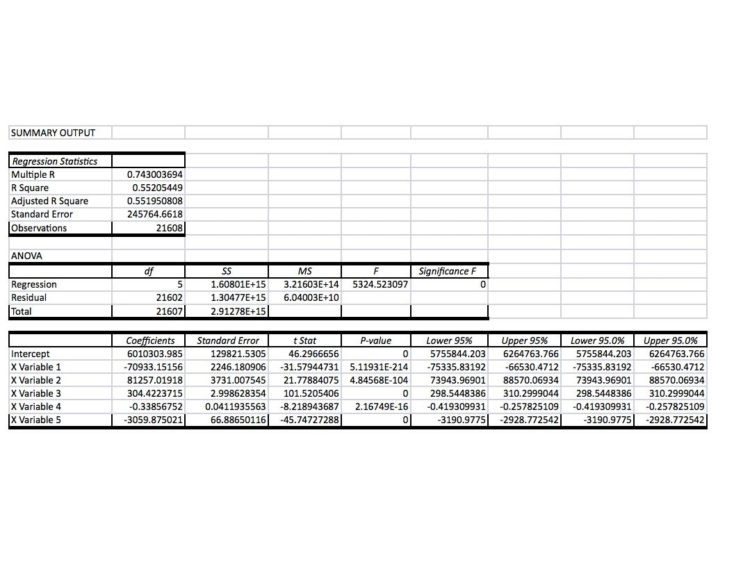
## Signif. codes:  0 '***' 0.001 '**' 0.01 '*' 0.05 '.' 0.1 ' ' 1

Here’s the corresponding output from Excel 2016 running under Parallels on an Apple laptop.

Excel Output

Let’s take the differences line-by-line

1. Summary Output: There may be an option tail to add it, but Excel doesn’t give you the formula for the model, the dependent and independent variables involved.
2. Excel analysis of variance (ANOVA), separately available in R is provided.
3. Regression Statistics:

• Excel adds “multiple R,” which is the square root of R Squared. It’s a measure of the goodness of predicting prices from the model, which can be calculated in R, but is not normally given in the output of the table. I couldn’t find any way in Excel of specifying whether to use Kendall’s tau or Spearman’s rho statistic.
• Excel’s remaining reports overlap those of R, except for the omission of detail of residuals and the F statistics.
• Excel adds confidence intervals, which are available in R separately. It’s not clear what the difference between the pairs of column represents, and the 95% confidence interval is normally expessed in terms of a value for 92.5% and 97.5%.
• Most of the results differ from those given my R for the same data. Except in the cases of the 0 valued p-levels for the t statistic, these are not large, and it is beyond the scope of my post here to figure out why. But apparently different computations are involved.